Predicting embryonic phenotypes of genetically modified zebrafish

In this tutorial, we predict perturbations on embryo-scale. Therefore, we consider ZSCAPE, which captures up to 23 perturbations at 5 different time points, resulting in 71 perturbed phenotypes. The experimental design is sparse, hence we investigate to what extent we can fill missing measurements with CellFlow’s predictions.

Preliminaries

The dataset is relatively large, hence we use rapids-single-cell which allows us to leverage GPU acceleration for preprocessing and downstream tasks. This notebook is executed on a A100 GPU with 80GB memory, as well as 500GB CPU memory.

import warnings
from pandas.errors import SettingWithCopyWarning

warnings.simplefilter("ignore", UserWarning)
warnings.simplefilter("ignore", FutureWarning)
warnings.simplefilter("ignore", SettingWithCopyWarning)

import numpy as np
import pandas as pd
import seaborn as sns
import jax
import functools
import matplotlib.pyplot as plt
import anndata as ad
import scanpy as sc
import rapids_singlecell as rsc
import flax.linen as nn
import optax
import cellflow
from cellflow.model import CellFlow
import cellflow.preprocessing as cfpp
from cellflow.utils import match_linear
from cellflow.plotting import plot_condition_embedding
from cellflow.preprocessing import transfer_labels, compute_wknn, centered_pca, project_pca, reconstruct_pca
from cellflow.metrics import compute_r_squared, compute_e_distance

/home/icb/dominik.klein/mambaforge/envs/cellflow/lib/python3.12/site-packages/optuna/study/_optimize.py:29: TqdmWarning: IProgress not found. Please update jupyter and ipywidgets. See https://ipywidgets.readthedocs.io/en/stable/user_install.html
  from optuna import progress_bar as pbar_module

adata = cellflow.datasets.zesta()

Let’s have a look at the most relevant columns:

• obs['timepoint'] the age of the embryo in hours post fertilization, as this covers a range from 18 to 72, we have created a columns "logtime" which stores the natural logarithm of "timepoint".

• obs['gene1+gene2'] contains the genetic perturbation, which can be a single or a double genetic knockout. CellFlow requires as many obs columns as the largest combination, which is 2 in our case. Hence, we created obs['gene_target_1'] and obs['gene_target_2'] which contain the single elements of the perturbation. Control cells have entries "control" in both columns, while single perturbations have "control" in obs['gene_target_2'].

• While not necessary for training CellFlow, it is handy to have obs['condition'], which contains the combination of the genetic perturbation and the time point.

• obs['is_control'] indicates whether a cell is a control cell. Note that we also have obs['first_t_control'], which we don’t need for the purpose for this notebook, but for Predicting the continuous, perturbed development of the zebrafish.

adata.obs.head()

	cell	Size_Factor	n.umi	perc_mitochondrial_umis	timepoint	Oligo	hash_umis	top_to_second_best_ratio	cell_type_sub	cell_type_broad	...	hash_plate	log.hash_umis	gene1+gene2	gene_target_1	gene_target_2	condition	is_control	first_t_control	logtime	germ_layer_adapted
A03_B01_P01-A01_LIG104	A03_B01_P01-A01_LIG104	0.766072	348.0	4.022989	18.0	18h_ctrl-inj_P13_H1	29.0	25.803177	head mesenchyme/PA cartilage	head mesenchyme/PA cartilage	...	NA	NaN	control+negative	control	control	control_control_18	True	True	2.890372	mesoderm_neural_crest
A03_B01_P01-A02_LIG101	A03_B01_P01-A02_LIG101	1.001617	455.0	9.010989	72.0	72h_ctrl-inj_P10_A6	46.0	5.384193	intestine (mid)	intestine	...	NA	NaN	control+negative	control	control	control_control_72	True	False	4.276666	endoderm
A03_B01_P01-A02_LIG127	A03_B01_P01-A02_LIG127	2.007637	912.0	1.644737	36.0	36h_ctrl-inj_P7_A8	15.0	9.082616	basal cell (early)	basal cell	...	NA	NaN	control+negative	control	control	control_control_36	True	False	3.583519	ectoderm_neural_crest
A03_B01_P01-A02_LIG257	A03_B01_P01-A02_LIG257	0.468889	213.0	0.938967	18.0	18h_ctrl-noto_P3_D7	24.0	21.347128	neural progenitor (hindbrain R7/8)	neural progenitor (hindbrain R7/8)	...	NA	NaN	control+negative	control	control	control_control_18	True	True	2.890372	ectoderm_neural_crest
A03_B01_P01-A03_LIG201	A03_B01_P01-A03_LIG201	0.537131	244.0	0.409836	48.0	48h_ctrl-noto_P16_H9	10.0	6.059433	neurons (differentiating, contains peripheral)	neurons (differentiating, contains peripheral)	...	NA	NaN	control+negative	control	control	control_control_48	True	False	3.871201	ectoderm_neural_crest

5 rows × 36 columns

We visualize the time point in hours post fertilization, and the genetic perturbation.

rsc.pp.neighbors(adata, use_rep="X_aligned")
rsc.tl.umap(adata)
sc.pl.umap(adata, color=["timepoint", "gene1+gene2"])

[2025-04-10 09:21:08.725] [CUML] [debug] n_neighbors=15
[2025-04-10 09:21:08.729] [CUML] [debug] Calling knn graph run
[2025-04-10 09:21:08.729] [CUML] [debug] Done. Calling fuzzy simplicial set
[2025-04-10 09:21:08.992] [CUML] [debug] Done. Calling remove zeros

Similarly to the use case in the CellFlow manuscript, we aim to predict the phenotype of a cdx4+cdx16 mutant at time point 36, which we first visualize:

custom_palette = {k: "#D6D6D6" for k in adata.obs["condition"].unique()}
custom_palette.update({"cdx4_cdx1a_36": "#CEA92D"})
order = list(adata[adata.obs["condition"] != "cdx4_cdx1a_36"].obs_names) + \
        list(adata[adata.obs["condition"] == "cdx4_cdx1a_36"].obs_names)

sc.pl.umap(
    adata[order],
    color="condition",
    groups=["cdx4_cdx1a_36"],
    palette=custom_palette,
    title="cdx4+cdx1a mutant at time point 36",
    size=10,
)

We split the data accordingly. Note that we need the control state at time point 36 also in the test data, to be able to translate these to their perturbed state.

adata_train = adata[adata.obs["condition"]!="cdx4_cdx1a_36"].copy()
adata_test = adata[(adata.obs["condition"]=="cdx4_cdx1a_36") | (adata.obs["condition"]=="control_control_36")].copy()
adata_train.n_obs, adata_test.n_obs

(2660905, 184343)

We use obsm['X_aligned'] as cellular representation, i.e. this is the space in which cells are generated. We note that the embedding was obtained from control cells only, with perturbed cells regressed onto it independently of other perturbed cells, such that we don’t have any data leakage from the test dataset. For details on the embedding, please refer to the ZSCAPE manuscript.

Setting up the CellFlow model

We are now ready to setup the CellFlow model.

Therefore, we first choose the flow matching solver. We select the default solver "otfm".

cf = CellFlow(adata_train, solver="otfm")

Preparing CellFlow’s data handling with prepare_data()

• As discussed above, we use obsm['X_aligned'] as cellular representation.

• obs['is_control'] indicates whether a cell is a control cell.

• perturbation_covariates indicates the external intervention, which is the genetic perturbation. As we also have combinations thereof, we pass the column names "gene_target_1" and "gene_target_2". We call this intervention "genetic_perturbation". We use ESM2 embeddings for representing the cytokines, which we have precomputed already for the purpose of this notebook, saved in uns['gene_embeddings']. Thus, we pass the information that "gene_embeddings" stores embeddings of the obs['cytokine'] treatments via perturbation_covariate_reps.

• The sample covariate describes the cellular context independent of the perturbation. We pass the time point via obs['logtime'].

• The split_covariates defines classes within which me map. As we want to learn maps from control to perturbed states within the same time point, we set "timepoint" to be the split covariate. See Predicting the continuous, perturbed development of the zebrafish for a different use of split_covariates.

• max_combination_length is the maximum number of gene knockouts seen during training or inference. We set it to 2. Note that this value is also automatically inferred from the maximum number of elements seen in perturbation_covariates, but can optionally set to be higher for inference.

• The null_value is the value which fills the absence of a perturbation, i.e. the value which fills all positions in uns['gene_embeddings']['control'].

cf.prepare_data(
    sample_rep = "X_aligned",
    control_key = "is_control",
    perturbation_covariates = {"genetic_perturbation": ("gene_target_1" , "gene_target_2")},
    perturbation_covariate_reps = {"genetic_perturbation": "gene_embeddings"},
    sample_covariates = ("logtime",),
    split_covariates = ["timepoint"],
    max_combination_length = 2,
    null_value = 0.0,
)

100%|██████████| 13/13 [00:02<00:00,  4.83it/s]
100%|██████████| 7/7 [00:01<00:00,  6.60it/s]
100%|██████████| 22/22 [00:04<00:00,  5.34it/s]
100%|██████████| 16/16 [00:02<00:00,  6.32it/s]
100%|██████████| 17/17 [00:02<00:00,  6.12it/s]

We now prepare the data validation data using prepare_validation_data().

As for some conditions, and in particular for control cells, we have a large number of measurements, we subsample for inference to be faster. However, due to the heterogeneity of the cellular distribution, covering hundreds of cell types, we should not subsample by too much.

adatas_train_subsampled = []
for cond in adata_train.obs["condition"].unique():
    adata_tmp = adata_train[adata_train.obs["condition"]==cond]
    adatas_train_subsampled.append(sc.pp.subsample(adata_tmp, n_obs=min(adata_tmp.n_obs, 10000), copy=True))

adata_train_for_validation = ad.concat(adatas_train_subsampled)

adatas_test_subsampled = []
for cond in adata_test.obs["condition"].unique():
    adata_tmp = adata_test[adata_test.obs["condition"]==cond]
    adatas_test_subsampled.append(sc.pp.subsample(adata_tmp, n_obs=min(adata_tmp.n_obs, 10000), copy=True))

adata_test_for_validation = ad.concat(adatas_test_subsampled)

As we require the embeddings for evaluation as well, we need to copy adata

adata_train_for_validation.uns = adata_train.uns.copy()
adata_test_for_validation.uns = adata_test.uns.copy()

cf.prepare_validation_data(
    adata_train_for_validation,
    name="train",
    n_conditions_on_log_iteration=10,
    n_conditions_on_train_end=10,
)

cf.prepare_validation_data(
    adata_test_for_validation,
    name="test",
    n_conditions_on_log_iteration=None,
    n_conditions_on_train_end=None,
)

100%|██████████| 13/13 [00:01<00:00,  8.78it/s]
100%|██████████| 7/7 [00:00<00:00,  8.82it/s]
100%|██████████| 22/22 [00:02<00:00,  8.83it/s]
100%|██████████| 16/16 [00:01<00:00,  8.89it/s]
100%|██████████| 17/17 [00:01<00:00,  9.01it/s]
100%|██████████| 2/2 [00:00<00:00, 221.14it/s]

Preparing CellFlow’s model architecture with prepare_model()

We are now ready to specify the architecture of CellFlow.

We only consider the most relevant parameters, for a detailed description, please have a look at the documentation of prepare_model() or Predicting donor-specific cytokine effects on PBMCs.

• We use condition_mode="deterministic" to learn point estimates of condition embeddings, and thus have a fully deterministic mapping. We set regularization=0.0, thus don’t regularize the learnt latent space.

• pooling defines how we aggregate combinations of conditions in a permutation-invariant manner, which we choose to do learning a class token indicated by "attention_token".

• With layers_before_pool we define how to embed the ESM2 embeddings and the log-value of the time. We process them such that have the same scale of dimensionality.

• condition_embedding_dim is the dimension of the latent space of the condition encoder.

• cond_output_dropout is the dropout applied to the condition embedding, we recommend to set it relatively high, especially if the condition_embedding_dim is large.

• pool_sample_covariates defines whether the concatenation of the sample covariates should happen before or after pooling, in our case indicating whether it’s part of the self-attention or only appended afterwards.

• probability_path defines the path between pairs of samples which the ConditionalVelocityField is regressed against. Here, we use {"constant_noise": 0.5}, i.e. we use a relatively small value as we have a highly heterogeneous cell population. In fact, if we augment a cell with noise, we should be careful not to augment it to the extent that it is e.g. in a completely different organ of the zebrafish.

• match_fn defines how to sample pairs between the control and the perturbed cells. As we have a strongly heterogeneous population, we choose a higher batch size of 2048. We don’t expect large outliers, and are not interested in the trajectory of a single cell, hence we choose tau_a=tau_b=1.0.

We start with defining the layers_before_pool and layers_after_pool.

layers_before_pool = {
    "genetic_perturbation": {"layer_type": "mlp", "dims": [512, 512], "dropout_rate": 0.0},
    "logtime": {"layer_type": "mlp", "dims": [512, 512], "dropout_rate": 0.0},
}

layers_after_pool = {
    "layer_type": "mlp", "dims": [1024, 1024], "dropout_rate": 0.0,
}

We now also explicitly define the match_fn:

match_fn = functools.partial(match_linear, epsilon=0.5, tau_a=1.0, tau_b=1.0)

Now we are ready to prepare the model:

cf.prepare_model(
    condition_mode="deterministic",
    regularization=0.0,
    pooling="attention_token",
    layers_before_pool=layers_before_pool,
    layers_after_pool=layers_after_pool,
    condition_embedding_dim=256,
    cond_output_dropout=0.9,
    hidden_dims=[2048, 2048, 2048],
    decoder_dims=[4096, 4096, 4096],
    probability_path={"constant_noise": 0.5},
    match_fn=match_fn,
    )

Computing and logging metrics during training

We compute the energy distance and MMD during training.

metrics_callback = cellflow.training.Metrics(metrics=["mmd", "e_distance"])
callbacks = [metrics_callback]

Training CellFlow

Finally, we are ready to train our model. We set the number of iterations relatively high as we have a strongly heterogeneous population.

cf.train(
        num_iterations=500_000,
        batch_size=2048,
        callbacks=callbacks,
        valid_freq=80_000,
    )

100%|██████████| 500000/500000 [4:21:28<00:00, 31.87it/s, loss=4.86]     

We can now investigate some training statistics, stored by the CellFlowTrainer.

e_distances_train = cf.trainer.training_logs["train_e_distance_mean"]
e_distances_test = cf.trainer.training_logs["test_e_distance_mean"]

iterations_train = np.arange(len(e_distances_train))
iterations_test  = np.arange(len(e_distances_test))

fig, axes = plt.subplots(1, 2, figsize=(18, 6))

axes[0].plot(iterations_train, e_distances_train, linestyle='-', color='blue', label='Energy distance training data')
axes[0].set_xlabel('Validation Iteration')
axes[0].set_ylabel('Energy distance')
axes[0].legend()
axes[0].grid(True)

axes[1].plot(iterations_test, e_distances_test, linestyle='-', color='red', label='Energy distance test data')
axes[1].set_xlabel('Validation iteration')
axes[1].set_ylabel('Energy distance')
axes[1].legend()
axes[1].grid(True)

Investigating the learnt latent space

We can visualize the learnt latent space for using get_condition_embedding().

covariate_data_train = adata_train[~adata_train.obs["is_control"].to_numpy()].obs.drop_duplicates(subset=["condition"])
covariate_data_test = adata_test[~adata_test.obs["is_control"].to_numpy()].obs.drop_duplicates(subset=["condition"])

df_embedding_train = cf.get_condition_embedding(covariate_data=covariate_data_train, condition_id_key="condition", rep_dict=adata_train.uns)[0]
df_embedding_test = cf.get_condition_embedding(covariate_data=covariate_data_test, condition_id_key="condition", rep_dict=adata_train.uns)[0]

df_embedding_train["seen_during_training"] = True
df_embedding_test["seen_during_training"] = False
df_condition_embedding = pd.concat((df_embedding_train, df_embedding_test))

100%|██████████| 16/16 [00:00<00:00, 607.06it/s]
100%|██████████| 21/21 [00:00<00:00, 653.02it/s]
100%|██████████| 6/6 [00:00<00:00, 641.15it/s]
100%|██████████| 15/15 [00:00<00:00, 659.43it/s]
100%|██████████| 12/12 [00:00<00:00, 654.27it/s]
100%|██████████| 1/1 [00:00<00:00, 467.75it/s]

fig = plot_condition_embedding(df_condition_embedding, embedding="PCA", hue="seen_during_training", circle_size=50)

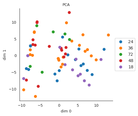
Now we can colorize it according to time point and genetic perturbation

df_condition_embedding["condition"] = df_condition_embedding.index
df_condition_embedding["genetic_perturbation"] = df_condition_embedding.apply(lambda x: "_".join(x["condition"].split("_")[:2]), axis=1)
fig = plot_condition_embedding(df_condition_embedding, embedding="PCA", hue="genetic_perturbation", circle_size=50)

df_condition_embedding["time_point"] = df_condition_embedding.apply(lambda x: x["condition"].split("_")[-1], axis=1)
fig = plot_condition_embedding(df_condition_embedding, embedding="PCA", hue="time_point", circle_size=50, legend=False)

Predicting with CellFlow

Predictions with CellFlow require an adata object with control cells. As we only want to generate cells corresponding the unseen perturbation cdx4 and cdx1a, we only need control cells for time point 36. Moreover, we require covariate_data to store the information about what we would like to predict.

adata_ctrl_for_prediction = adata_test[(adata_test.obs["is_control"].to_numpy()) & (adata_test.obs["timepoint"]==36)]
covariate_data = adata_test[~adata_test.obs["is_control"].to_numpy()].obs.drop_duplicates(subset=["condition"])
covariate_data

	cell	Size_Factor	n.umi	perc_mitochondrial_umis	timepoint	Oligo	hash_umis	top_to_second_best_ratio	cell_type_sub	cell_type_broad	...	hash_plate	log.hash_umis	gene1+gene2	gene_target_1	gene_target_2	condition	is_control	first_t_control	logtime	germ_layer_adapted
A03_B01_P01-A02_LIG135	A03_B01_P01-A02_LIG135	3.180959	1445.0	16.33218	36.0	36h_cdx4-cdx1a_P2_G7	31949.0	inf	mature slow muscle 3	mature slow muscle	...	P2	4.504457	cdx4+cdx1a	cdx4	cdx1a	cdx4_cdx1a_36	False	False	3.583519	mesoderm_neural_crest

1 rows × 36 columns

We specify sample_rep to be "X_aligned", and provide a condition_id_key which defines the keys of the returned dictionary containing the predictions.

preds = cf.predict(adata=adata_ctrl_for_prediction, sample_rep="X_aligned", condition_id_key="condition", covariate_data=covariate_data)

100%|██████████| 1/1 [00:00<00:00, 462.28it/s]

We now build an adata object to store the predictions in adata.obsm:

adata_preds = []
for cond, array in preds.items():
    
    obs_data = pd.DataFrame({
        'condition': [cond] * array.shape[0]
    })
    adata_pred = ad.AnnData(X=np.empty((len(array),adata_train.n_vars)), obs=obs_data)
    adata_pred.obsm["X_aligned"] = np.squeeze(array)
    adata_preds.append(adata_pred)

adata_preds = ad.concat(adata_preds)
adata_preds.var_names = adata_train.var_names

We now transfer labels using the 1NN classifier based on the training data. Therefore, we first have to compute a nearest neighbor graph, and then transfer the labels subsequently.

compute_wknn(ref_adata=adata_train, query_adata=adata_preds, n_neighbors=1, ref_rep_key="X_aligned", query_rep_key="X_aligned")
transfer_labels(query_adata=adata_preds, ref_adata=adata_train, label_key="cell_type_broad")

adata_preds.obs["mode"] = "generated"
adata_train.obs["mode"] = "train"
adata_test.obs["mode"] = "test"

adata_concatenated = ad.concat((adata_preds, adata_train, adata_test[~adata_test.obs["is_control"].to_numpy()]))

rsc.pp.neighbors(adata_concatenated, use_rep="X_aligned")
rsc.tl.umap(adata_concatenated)

[2025-04-10 14:24:46.742] [CUML] [debug] n_neighbors=15
[2025-04-10 14:24:46.849] [CUML] [debug] Calling knn graph run
[2025-04-10 14:24:46.849] [CUML] [debug] Done. Calling fuzzy simplicial set
[2025-04-10 14:24:47.464] [CUML] [debug] Done. Calling remove zeros

For a visual assessment, we compare true cells with generated cells on a UMAP

adata_concatenated.obs["condition_mode"] = adata_concatenated.obs.apply(lambda x: x["condition"] + "_" + x["mode"], axis=1)
adata_concatenated.obs.reset_index(inplace=True)

color_palette = {"generated": "#B12F8C", "test": "#3F8AA6", "train": "#B6B6B6"}
order = list(adata_concatenated[adata_concatenated.obs["mode"]=="train"].obs_names) + list(adata_concatenated[adata_concatenated.obs["mode"]=="generated"].obs_names) + list(adata_concatenated[adata_concatenated.obs["mode"]=="test"].obs_names)
sc.pl.umap(adata_concatenated[order], color=["mode"], palette=color_palette, size=10)